


Introduction
Testing materials of construction for use in wells with corrosive production fluids is typically accomplished through autoclave (pressure vessels) experiments. This testing is important because production fluids contain a combination of acid gases (CO2 and H2S), salts, and elevated temperature and pressure conditions [1]-[2].
These autoclave experiments replicate the fluid environment that the materials of construction will encounter, replicating the downhole environment, including the CO2 and H2S acidity, the water phase salinity, and the downhole temperatures. Materials tested are generally some form of corrosion-resistant, high-nickel alloys (CRAs) [3].
As the industry moves towards deeper wells, the operation conditions change:
- T =150 – 260 ⁰C (302 to 500 ⁰F)
- P = 1000 to 2400 bar (14500 to 35000 psi)
- Concentration of dissolved solids: TDS> 300,000 mg/L
- High partial pressure of dissolved gases such as CO2 and H2S
These conditions induce scaling and severe corrosion damage to construction metals in wells.
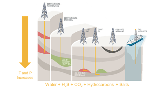
Figure 1. Scaling and corrosion damage issues are exacerbated as the industry moves towards deeper wells.
Recreating the downhole environment is difficult because well pressures, sometimes >1000 bar, cannot be recreated in an autoclave experiment. These pressures impact fluid chemistry significantly. They affect concentrations of molecular CO2 and H2S in the brine phase. These concentrations dominate the susceptibility of a CRA to corrosion.
Thus, there is an essential need to translate the downhole fluid environment into a laboratory autoclave environment. OLI simulation software accomplishes this by computing the key properties of downhole fluids and converting this to an autoclave formulation that will achieve the same properties. These include pH, chloride activities, molecular CO2 and H2S activities, and if possible, the bicarbonate activities. Activity is a thermodynamic property that relates the measured concentration to its actual reactivity in the water phase. There are several references that describe how these activities are calculated and why they are a better representation of corrosivity than the actual concentration value. This is the case not just for corrosion but also solid solubility, boiling point, and other measurable properties.
OLI calculates these activities using a comprehensive thermodynamic framework, referred to as the MSE-SRK model. This model is used for simulating fluids containing H2S, CO2, H2O, hydrocarbons, and salts at high temperatures and pressures [4].
This MSE-SRK model is coupled with the OLI Flowsheet simulation tool to 1) calculate the fluid properties at downhole conditions, and 2) develop autoclave recipes that recreate these downhole properties. These recipes are based on achieving target concentrations of key gases (CO2 and H2S) in water, pH, or other properties critical to the autoclave experiment. It is important to note that other properties, such as activities and concentrations of key species in solution, as well as partial pressures and fugacities of aggressive species, can also be calculated.
The MSE-SRK thermodynamic framework when combined with a simulation tool such as OLI Flowsheet: ESP helps to:
- Predict phase equilibria including supercritical and subcritical states in multiphase and multicomponent systems
- Understand the partitioning and speciation of aggressive species such as CO2 and H2S
- Account for non-ideality effects, to accurately predict activities (in the brine) and partial pressures and fugacities (in the vapor phase) of aggressive species in a downhole environment
- Accurately predict production fluids properties such as pH and saturation indexes (SI)
Autoclave Testing
Laboratory testing standards are available to evaluate the corrosivity of production fluids on materials of construction [5]. Proper testing must be performed before materials are approved for service.
Designing the material testing environment depends entirely upon the intended application of the material. Downhole environments vary considerably in H2S, CO2, and Cl– concentration; downhole temperatures and pressures also vary depending upon the reservoir and location in the well. The environmental parameters that must therefore be simulated are the partial pressures or fugacities of the cover gases (H2S and CO2), temperature, and the chloride content (Cl–).
A typical range of downhole environments in oil and gas wells is summarized in Table 1.
Table 1. Typical range of downhole environment in oil and gas wells [6]
| Parameters | Oil Wells | Gas Wells |
| Temperature of Wellhead, °C | 38-66 | 38-135 |
| Temperature at Bottom of well, °C | 38-121 | 121-260 |
| Total Pressure, atm | 136-531 | 293-1565 |
| Partial Pressure of H2S, atm | 0-14 | 0-544 |
| Partial Pressure of CO2, atm | 0-14 | 0-204 |
| Chloride concentration | 0 to saturation | 2 wt% to saturation |
Why use simulation for autoclave experiments?
A limiting condition of autoclave experiments is that once the autoclave is sealed and at test conditions (pressure and temperature), it is difficult and sometimes impossible to sample and measure the final phase compositions within the vessel. Consequently, one cannot know for sure if the experiment meets the field conditions.
This uncertainty is reduced by using OLI thermodynamic simulations. OLI Flowsheet calculates the critical concentrations and properties at field conditions and converts them to a laboratory formulation. This achieves a number of benefits, including the ability to:
- Predict the required gas partial pressures in the autoclave at test conditions
- Predict aqueous phase properties, such as pH, alkalinity, conductivity, osmotic pressures
- Predict CO2 and H2S partitioning across a fluid phase (oil, gas, and water)
- Predict solids formation (e.g., FeS, FeCO3, CaCO3) that may affect the final properties
- Predict the species concentrations in the water
- Create a recipe for the autoclave experiment, i.e., grams of CO2 H2S, N2, water, salt, etc. that will be added to autoclave
Case Study
An oil and gas operator wants to test the corrosivity of a production gas/brine on their production tubing. The production conditions are 350 bar and 150 ⁰C. The partial pressures of CO2 and H2S are 20 bar and 1 bar, respectively. The produced water is simulated using a 50,000 mg/L NaCl solution. The operator needs to charge the autoclave with sufficient CO2 and H2S so that at the final conditions, their vapor concentrations match the measured values.
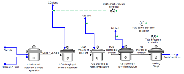
The simulation is broken down into 5 different steps needed to sequentially charge the autoclave to reach the final T and P conditions, as shown in Figure 2. These steps all represent the same autoclave vessel. Step 1 represents the placement of the sample (with its respective volume) and the addition of the deaerated brine volume. Step 2, 3, and 4 represent charging the autoclave with CO2, H2S, and N2, respectively, at ambient conditions. Step 5 represents heating to reach the final temperature and pressure, and the desired final partial pressures of the acid gases.
You can see that the targeted partial pressures were achieved in the simulation, i.e. partial pressures of CO2 and H2S are 20 bar and 1 bar, respectively. To reach these values the CO2 and H2S inflows need to be 9.02 L/h and 0.59 L/h, respectively. After reaching the final T=150°C and P=350 bar, you can also see the final predicted pH value and fugacities of the acid gases.
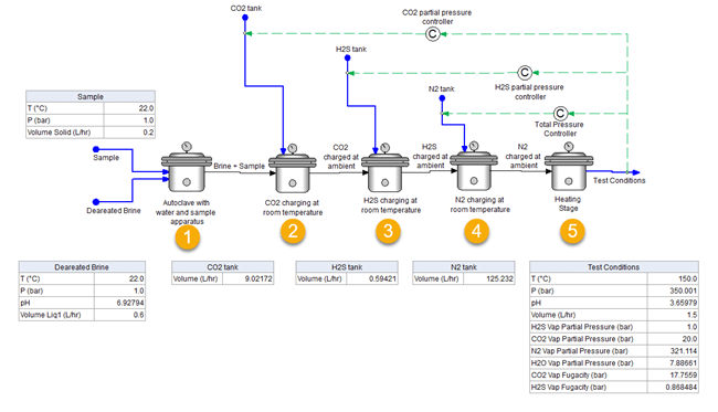
Figure 2. Sequential autoclave charging procedure for case study
Autoclave Configurations and how to simulate them with OLI Flowsheet: ESP Software
When working with autoclaves, there are several experimental autoclave charging procedures. With the OLI Flowsheet: ESP software you have the flexibility to recreate your autoclave charging procedure and determine the autoclave recipe (gas amount or bottle gas composition) needed to reach your final conditions. Here we will describe six different autoclave procedures that can be simulated; however, the options, of course, are unlimited.
- Final Condition Autoclave – The most common autoclave used by customers is the final condition autoclave. It is the basic configuration, in which the test solutions and the gases are added in a single step, and the properties and concentrations are computed. The image below shows two solutions, a brine and gas are added simultaneously with CO2 and H2S. The vessel is at test temperature, and the test pressure is calculated. The mass (or volume) of the brine and oil are known. The amounts of CO2 and H2S to be added are calculated using the PCO2 and PH2S targets.
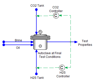
The purpose of the Final Condition Autoclave is to calculate the mass requirements for the experiment (i.e., the recipe). This does not include the actual procedure.
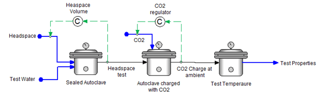
2. Autoclave Charging with CO2 to Set the Final Pressure
This next example is based on an autoclave charging procedure in which the test solution is added to the sealed autoclave, and the remaining purge gas occupies the headspace. The sealed autoclave is then charged with CO2. The amount of CO2 added depends on the target total pressure at ambient conditions. The autoclave is heated to test temperatures and the test pressure and CO2 partial pressures are computed.
3. Sequential Charging of Gases
This next example uses three pure gases, CO2, H2S, and N2. This is the same charging procedure as shown in Figure 2. The amount of each gas added is based on achieving a target PCO2, PH2S, and PT. The gases are added in sequence at ambient temperature. The vessel pressure after each charging step is computed and this pressure value sets the gas tank regulators in the laboratory.
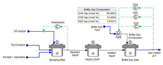
4. Bottle Gas Charging
This next example is for charging an autoclave when a bottle gas is used. The advantage of this simulation is that the composition of the bottle gas can be computed based on the PCO2, PH2S, and PT targets. The software calculates the mole fraction of the bottle gas using three composition controllers. These controllers measure the partial pressures at test temperature and modify the composition. The laboratory can then order this gas from the supplier.
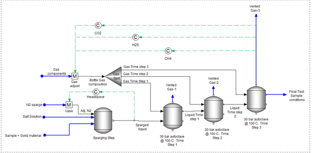
5. Bottle Gas Continuously Bubbled at Test Conditions
This next configuration simulates an open autoclave experiment. In this case, bottle gas is bubble continuously into the vessel. The amount of gas required to reach steady-state conditions is computed. The purpose of this procedure is to provide a reasonable estimate of how much time is required for the system to reach target conditions.
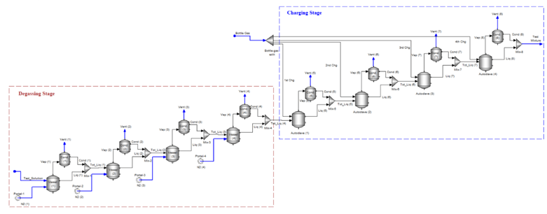
6. Degassing Stages before Charging Gases
This next configuration is a combination of purging and charging for a continuous bubbling system. The N2 degassing step provides a reasonable estimate of how much volume (or time) is needed to purge O2 to its desired concentration. The charging step, as above, simulates the amount of time (or volume) needed for the gases to reach an equilibrium steady-state with the liquid in the autoclave. The degassing step is run at ambient temperatures while the charging step is run at test temperatures.
These are a few examples, of the many ways autoclaves experiments can be simulated. You can always ask for an autoclave template to get you started with your simulation. You can download the technical whitepaper on autoclave simulation here https://www.olisystems.com/autoclave-charging.
For more information on the OLI Software Platform V10 visit https://www.olisystems.com/oli-platform-v10 and for more information OLI products visit https://www.olisystems.com/products
Please contact Diana Miller, Application Engineer and Autoclave Simulation Expert at OLI Systems at diana.miller@olisystems.com for more details on OLI’s autoclave testing capabilities. To speak to an OLI technical or sales specialist please register your interest at https://www.olisystems.com/contact or email sales@olisystems.com
Bibliography
- 1] T. E. Perez, “Corrosion in the oil and gas industry: An increasing challenge for materials,” Jom, vol. 65, no. 8, pp. 1033–1042, 2013.
- [2] L. T.Popoola, A. S. Grema, G. K. Latinwo, B. Gutti, and A. S. Balogun, “Corrosion problems during oil and gas production and its mitigation,” Int. J. Ind. Chem., vol. 4, no. 35, 2013.
- [3] M. Ueda, “2006 F.N. Speller Award Lecture: Development of corrosion-resistance alloys for the oil and gas industry – Based on spontaneous passivity mechanism,” Corrosion, vol. 62, no. 10, pp. 856–867, 2006.
- [4] R. Springer, A. Anderko and D. Miller, “ MSE-SRK: A Thermodynamic Model to Maximize the Accuracy of Predicting Phase Equilibria in Systems Containing Sour Gases, Electrolytes, and Hydrocarbons”, Nashville, TN: NACE, RIP Section, 2019
- [5] “NACE MR0175/ISO 15156-2, Petroleum and natural gas industries- Materials for use in H2S-containing environments in oil and gas production.,” Houston, TX: NACE, 2009.
- [6] R. D. Mack, M. Wilhelm, and B. G. Steinberg, “Laboratory Corrosion Testing of Metals and Alloys in Environments Containing Hydrogen Sulfide,” in Laboratory Corrosion Tests and Standards, American Society for Testing and Materials, 1985, pp. 249–250.