


New OLI Optimizer tool for OLI Flowsheet: ESP V11 maximizes performance of assets and processes to accelerate the industrial digital transformation
Process Optimization in Chemical Engineering
In chemical engineering, optimization is typically used to either maximize or minimize an objective function which links the variable that needs to be optimized with the design and operating variables. Since engineering problems may have multiple solutions, the goal very often is to select the option which comes closest to maximizing the economic performance. To optimize the process, it becomes important to identify the objectives, constraints, and degrees of freedom in the process to achieve benefits such as improving the design quality, ease of trouble shooting and provide a quick way to make the right decisions [1].
Optimization can take place at any level across the various process steps ranging from a complex combination of all systems and sub-systems of process steps and equipment (global optimization) or it can be confined to a specific piece of equipment of smaller units (local optimization). In addition to optimizing a process, the same approach can also be used to calibrate first principles-based simulation models for specific assets or processes which will enable more accurate model prediction [1].
OLI software platform provides unique data properties and simulation software innovations to tackle complex water chemistry-based operations challenges in oil & gas, water treatment, mining, power generation and chemicals industries. OLI software platform also provides an excellent foundation to deliver flowsheet model optimization to optimize chemical processes. OLI Systems has developed a general-purpose optimization capability to use in process flowsheeting software aka OLI Flowsheet: ESP. This capability will be available in the upcoming OLI Platform V11 release expected in the end of Q1 2021. Along with OLI Optimizer tool, the new OLI platform V11 will also deliver cloud apps, cloud APIs and bulk data input capabilities to fuel the industrial digital transformation.
In this article, we discuss the scope of the optimization capabilities that will become available in the OLI V11 platform and provide some simple, illustrative examples of these new capabilities.
Scope of optimization in the OLI Platform V11
The optimization feature will enable users to optimize flowsheet for process variables (parameters for streams and unit operations/blocks), kinetic parameters and some thermodynamic parameters of OLI’s MSE and Aqueous framework.
Table 1: Optimization scope in OLI Flowsheet: ESP for our next V11 release
| Optimization scope | Type | Description |
| Process variables | Stream parameters | Any stream input parameters |
| Block parameters | Any block input parameters | |
| Thermodynamic parameters | UNIQUAC interactions | UNIQUAC, extended UNIQUAC and pressure dependent UNIQUAC |
| Midrange interactions | Midrange and pressure dependent midrange | |
| SRK interactions | Mixing rule parameters, Kabadi-Danner coefficient¥ | |
| Kfit coefficients | Temperature and pressure dependent parameters | |
| Pitzer interaction¥ | Ion-molecule, molecule-molecule interaction | |
| Bromley interaction¥ | Ion-ion interaction | |
| Kinetic parameters | Std or Arrhenius | Arrhenius rate equation |
| User-defined | User defined rate equation | |
| ¥ for AQ framework only or not used in MSE framework | ||
Optimization options:
OLI is using derivative-free bound-constrained optimization algorithm from nonlinear optimization (NLOPT) library. NLOPT is a free/open-source library for nonlinear optimization, providing a common interface for several different free optimization routines available online as well as original implementations of various other algorithms. NLOPT provides a common interface for many different algorithms. NLOPT is a free/open-source software under the GNU LGPL (and looser licenses for some portions of NLOPT) license.
Table 2: Optimization options in OLI Flowsheet: ESP for our next V11 release
| Options | uses |
| Objective weight | Users may set weight to tilt the objective |
| Initial value | Required to provide initial values |
| Upper and lower bounds | Recommended, if available |
| Fix or Free | Users set “free” for varying, “fix” to use the value as is in optimization |
| Initial step | Users may provide if information available |
| Maximum evaluation | There is default, users may override |
| Function scaling | For multi-objectives, when objectives are different order of magnitude |
| Run affected blocks only | Runs blocks/streams that are tied to objectives/variables, saves time |
| Stopping criteria | Many stopping criteria, absolute/relative error, stopping at certain value |
Optimization applications:
Here, we are providing three simple examples to display the rigor of optimization capability in OLI Flowsheet: ESP. A block parameter manipulation, thermodynamic interaction manipulation and a standard kinetic equation parameter manipulation to reach a specific target. These applications are hypothetical and simple, yet users will be able to optimize simple cases like these, overly complicated cases and complex chemistries. A more detailed description of the feature with many interesting applications will be presented in a separate blog.
Example 1: Block parameters – simple
A user wants to identify the flowrate of NAC6H11O7 (sodium gluconate) for which the maximum concentration of NDC6H11O7ION e.g., Neodymium(III) gluconate ion(+2) exists in “Output” stream.
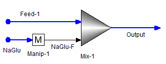
The user set the optimizer the following way. Only 1 objective which is to maximize concentration of NDC6H11O7ION in the “Output” stream. The stream “NaGlu” contains only NAC6H11O7. The vary variable (only 1 here) is set as to vary the manipulator (Manip-1) total flow factor.
Table 3: Optimizer settings for example-1
| Objectives | Value | |
| 1 | Objective 1 | Maximize, NDC6H11O7ION in “Output” |
| Variables | ||
| 1 | Vary variable object, Block variable | Manip-1, Total flow factor |
| Type | Free | |
| Initial value | 0.5, Set by user (always required) | |
| Minimum value | 0.0, Set by user | |
| Maximum value | 1.0, Set by user | |
| Options name | ||
| fTol_abs (abs tol on function value) | 1.0E-4 | |
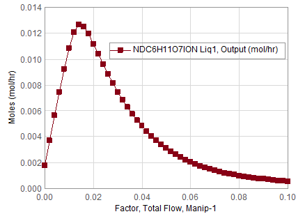
The optimization returns the above in block output window and it finds the manipulator (Manip-1) total flow factor as 0.01475 for which the concentration of NDC6H11O7ION in the “Output” stream is maximum of 0.0126851 mol/hr. To confirm, user conducted a sensitivity analysis or survey in either OLI Flowsheet or OLI Studio and finds that a maximum exists near that region.
Example 2: Thermodynamic – Midrange parameters
Let us take a hypothetical case, the “Feed-1” stream remains as it is in Example-1; the “NaGlu” stream contains only 0.014 mole/hr of NAC6H11O7. After equilibrium, user finds that “Output” stream contains 0.01266 mol/hr of NDC6H11O7ION and 1.16049E-3 mol/hr of NDION (true species). Let us assume, from experience or from plant data, user knows at the temperature, pressure, and concentrations, it is highly unlikely to have any NDC6H11O7ION and more of NDION should exist. The user now wants to modify the chemistry aka the thermodynamic parameters behind it so that trace or none NDC6H11O7ION in the speciated true species. The user decided to adjust midrange interaction between NAION and NDC6H11O7ION. The user thinks of adjusting BMD0, BMD1, BMD2 between the two ions.
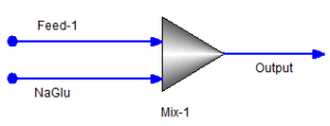
Table 4: Optimizer settings for example-2
| Objectives | Value | |
| 1 | Objective 1 | Minimize, NDC6H11O7ION in “Output” |
| Variables | ||
| 1 | Vary variable object, Thermo – MIDRANGE | BMD0, NAION/NDC6H11O7ION |
| Type | Free | |
| Initial value | -90.0, Set by user (always required) | |
| Minimum value | Default | |
| Maximum value | Default | |
| 2 | Vary variable object, Thermo – MIDRANGE | BMD1, NAION/NDC6H11O7ION |
| Type | Free | |
| Initial value | 0.5, Set by user (always required) | |
| Minimum value | Default | |
| Maximum value | Default | |
| 3 | Vary variable object, Thermo – MIDRANGE | BMD2, NAION/NDC6H11O7ION |
| Type | Free | |
| Initial value | 1000.0, Set by user (always required) | |
| Minimum value | Default | |
| Maximum value | Default | |
| Options name | ||
| fTol_abs (abs tol on function value) | 1.0E-6 | |
Optimization succeeded in 10 iterations with NDC6H11O7ION of 6.725E-8 mol/hr and NDION of 0.00767 mol/hr, respectively. Concentration of NDC6H11O7ION is now trace, whereas concentration of NDION increases substantially. BMD0, BMD1 and BMD2 converged to -88.8601, -1.00032 and 1003.73, respectively. It is to be noted that there are risks involved using local model and it is recommended to apply due diligence while using local model for simulation/design purposes. Please consult with experienced professionals and/or OLI experts for data optimization.
Example 3: Kinetic – std parameters
Let us consider a case of using reaction kinetics for the hydrolysis of urea. Urea is kinetically controlled, and the kinetic equation is provided as below
![]()
And the standard kinetic parameters are KF = 20.0, AR = 1.2E-6, BR = 3480.78, and EP2 = 0.0. On the reactor block, the number of stages and residence time are chosen as 10 and 100 hr, respectively. Let us assume the inflow to the reactor block “Feed” contains 6.8965 mol/hr CO2 and the user wants to achieve 45% on apparent molecular basis UREA in “Product” stream while considering CO2 as the limiting reactant e.g., that calculates to 3.10 mol/hr CO2 on apparent molecular basis. The user wants to vary the forward reaction rate constant, KF.
Table 5: Optimizer settings for example-3
| Objectives | Value | |
| 1 | Objective 1 | Minimize, (UREA – 3.10) in “Product” |
| Variables | ||
| 1 | Vary variable object, Kinetic-std | KF |
| Type | Free | |
| Initial value | 1.0E8, Set by user (always required) | |
| Minimum value | 1.0E6, Set by user | |
| Maximum value | 1.0E12, Set by user | |
| Options Name | ||
| fTol_abs (abs tol on function value) | 1.0E-6 | |
Here, the user provided both upper and lower bound for KF. Since, KF must be a positive value for UREA formation, the user may only provide a lower bound of some positive value and keep the upper bound off from the calculation options. The software will default to upper or lower bound value if not provided, but users may have more firsthand information than the software does. The calculation completes in 23 iterations with KF value being 1.91772E9 and the UREA in “Product” stream of 3.10 mol/hr.
In the last two examples, we explored how optimization can be taken to the molecular interaction and kinetic reactions level. This is important in multiple levels. The ability to take in plant data and “calibrate” interaction and kinetic parameters allows processes to be modeled to react just as the real process would. Model calibration enables “process” optimization that will have real-life results. Once the model is calibrated, studies can be performed in the model to maximize production and minimize inputs and energy consumption. Thus, model calibration enables the business unit to efficiently, and safely, increase the unit’s bottom line by increasing throughput and efficiency as well as by lowering operating costs, increasing reliability, and eliminating unplanned downtime.
Please tune in for more interesting applications which will be presented in an upcoming blog post. OLI Systems would like to work with clients in optimizing their flowsheet applications and our experienced team of Application Engineers and Consultants will be glad to discuss this further.
OLI Systems offers a unique combination of material properties, models and software that uses first principles based thermodynamic and electrochemical modeling. The OLI property database of over 6,000 species covers over 80 elements of the periodic table. OLI’s physical property methods, and property parameters and data are the ideal choice to suit your simulation needs. OLI Systems has expert scientists, thermodynamicists, engineers and consultants ready to help your thermodynamic data development, defining complex chemistry, conducting sponsored-research and Joint Industry Programs (JIPs) for industrial water and electrolyte chemistry applications.
Contact OLI for more information or to schedule a meeting with an OLI expert.
References:
- Gil Chavez et. al., 2016. Process Optimization in Chemical Engineering. In: Gil Chavez et. al. (Ed.), Process Analysis and Simulation in Chemical Engineering, Springer International Publishing, Switzerland, pp. 343-369.


