


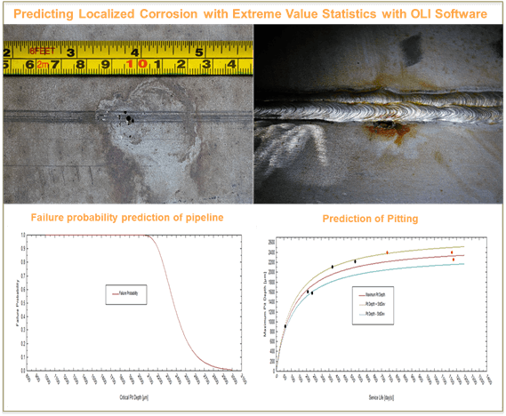
 Types of Corrosion Damage
As is well known, corrosion damage can be classified into two categories: uniform (general) corrosion and localized corrosion, and the quantitative description of these two cases is quite different. In the case of general corrosion, it is natural to define corrosion damage at a given point on a metal surface as being the thickness of the metal layer that has corroded, a. This definition means that we can predict general corrosion damage if we can calculate a as a function of time and of the independent variables controlling the damaging process. Even the term ‘uniform corrosion’ shows that, usually, the corroding layer thickness, a, depends slightly on the coordinates on the metal surface, if internal and external variables can be considered to be approximately constant for different parts of the system.
On the other hand, in the case of localized corrosion, the situation becomes more complicated. Generally speaking, the accumulation of localized corrosion damage in a system is completely defined if we know how many pits or other corrosion events (per square centimeter) have depths between x and x +dx for a given observation time, t, at a given location on the metal surface. However, in the overwhelming majority of practical cases, such complete information is not required to effectively predict the failure time due to the penetration of the deepest event. Thus, very often, it is sufficient to obtain information about only the deepest corrosion event (pit, crack), because failure in the system commonly occurs when the depth of the deepest corrosion event amax exceeds some critical value, acr. Usually, acr is the thickness of the wall of a pipe, for example, or the depth of a pit transitioning into an unstable crack.
The problem is that acr can be quite different in different parts of the system in spite of the fact that the parts can be under practically the same environmental conditions. Thus Figure 1 shows the typical data for the depths of the deepest pit experimentally measured on 9 sample areas (50×50 cm) on the outer surface of the underside of a tank having total surface area 175 m2 of carbon steel, storing heavy petroleum, after 20 years of service. The thickness of the wall is 6 mm.
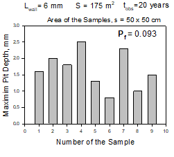
As we can see the difference between different values of amax range over 300 % for this example. This is the sequence that characterizes corrosion processes that depend on a series of complicated factors in a very complicated manner. Practically it means that prediction of localized (pitting) corrosion damage must be done in probabilistic terms as it was pointed out as early as the 1930s by U. R. Evans. Thus, for the current system the practical questions are (1) what is the probability, Pf, that the leaks in the tank can exist at the time of observation and (2) to predict how this probability changes with time.
Extreme Value Statistics
The answer to the first question can be formulated by using a purely mathematical approach, namely the Extreme Value Statistics (EVS) which is a branch of statistics dealing with the extreme deviations from the median of probability distributions. As applied to corrosion problems EVS have been used extensively to extrapolate damage (maximum pit depth) from small samples (in the laboratory or in the field) to larger area samples in the field (see Kowaka et al. 1994). Thus, it was shown that probability of failure of a construction, Pf, i.e. the probability that at least one pit reaches the critical dimension, acr, (for example wall thickness) in the system with area S is described by the equation:
![]() (1)
(1)
where location parameter, u, and scale parameter, α, are measured by using small samples with area, s. Equation (1) is to extrapolate corrosion damage from a small reference area, such as a coupon to a larger operational area, S. This is the classical use of Extreme Value Statistics. Thus, calculations performed for the extreme pit distribution shown on Figure 1 yield for the probability of leaking, Pf = 0.093, at observation time t = 20 years.
It is evident that in order to predict how this probability of failure, Pf(t), changes with time we need to assume how parameters u and α change as functions of time and experimental studies demonstrate that both the shape and location parameters are time-dependent. However, those dependencies must be established empirically or theoretically (by using adopted physicochemical models) and since no theory contained within classical EVS is available for the functional forms of u(t) and α(t), it is necessary to know these functions in advance for predicting the damage at long times. This has proven to be a severe constraint on the applicability of classical EVS.
Generally speaking, in the case of an empirical approach (which is used in OLI Software Platform EVS module) such dependencies can be established by assuming some analytical relations for u(t) and α(t) containing some unknown parameters and these parameters can be fitted to experimental distributions of deepest pits with some mean value, μ, and the standard deviation from extreme pits depth, σ. In accordance with EVS, μ, are functions of time and area of the system:
μ(t,S) = u(t) + α(t)[E + ln(S/s)] and σ(t) = α(t)π/√6 (2)
where E = 0.5772 is Euler’s constant. It is clear that measurements for at least two different times must be performed for establishing the fitting process.
One of the unique capabilities in the OLI software platform is the ability to estimate EVS parameters
It is clear that the choosing of assumed analytical forms for u(t) and α(t) is a question of a great importance. The typical time-relations that are usually used for estimating the location and scale parameters in extreme value distributions are of the power law type:
![]() ,
, ![]() (3)
(3)
where, a1, a2, and a3 are unknown parameters that must be determined by fitting Expressions (2) to short-term experimental data. Relation for u(t) in the form of power function is usually justified by the experimentally observed power law of mean pit depth as a function of time. As mentioned by [Laycock et al. 1990], the value a2 = 1 is often used by default, in particular when reference is made to an (implicitly constant) “pitting rate” of, say, “1 mm per year.”
On the other hand, some different simple analytical relations for u(t) and α(t) can be obtained by applying damage function analysis (DFA) method that considers propagation of corrosion damage by drawing an analogy between the growth of a pit and the movement of a particle (Engelhardt and Macdonald, 2004). Thus, the inclusion of the delayed repassivation phenomenon (sometimes referred to as “stifling”) and assuming “instantaneous nucleation” of pits leads an analytical expression for u and α in terms of time of the hyperbolic form:
![]() ,
, ![]() (4)
(4)
Namely, equations (3) are used now by OLI software for predicting damage in corroding systems.
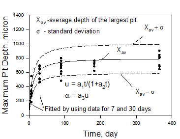
It must be noted that any Equations (3) or (4) (and some other equations) can adequately describe already known experimental data by corresponding fitting parameters a1, a2 and a3. Let us consider, for example, data from classical experiments performed by Aziz (1956) on Alcan aluminum alloy 2S-O in Kingston tape water (see Figure 2).
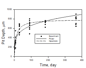
However, for practical purpose it is much more important to predict the results of long-time experiments (the propagation damage into future) by using for fitting only the data obtained in short term experiments (already known). Figures 3 and 4 namely show predictions of the depth of the deepest pit of long-time experiments (up to 1 year) by using data only of short-time experiments (t = 1 week and 1 month).
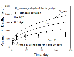
As we can see the hyperbolic dependence of fitted coefficients accepted in the OLI software provides (Figure 4) an accurate extrapolation over a range of 12 times that of the calibration range. On the other hand, application of the power law functions for fitting experimental data to the short-term experiments yields results that are not as good as given by the hyperbolic law, at least for the considered experimental data. This happens, because the power law does not take into account the repassivation of pits that plays a substantial role in determining the results of Aziz’s experiments. It means that hyperbolic law for presenting u(t) (that is used in OLI software) for predicting pitting damage mainly more acceptable (has more predictive power) than usually used power law.
Input and Output
For applying this technique the user has to provide a set of experimental data (xi, ti, si), i = 1,2,…,N, where xi is the depth of the deepest pit over area si, of a metal exposed to corrosion attack. The separate area, si, could be distinct coupons (in general case, with different area) from a designed experiment or random samples at various times from different locations in the system. Experiments must be performed for at least two different times.
The output of the code yields:
Depth of the deepest pit (with the standard deviation) in the engineering structure or laboratory systems as a function of time, t, and the surface area, S of the system.
These data are useful for comparison with experiments.
In addition, the code allows one to perform important engineering calculations, such as
(a) Probability of failure, Pf, for a given critical penetration depth, acr, (for example wall thickness) and the area of the system, S, as a function of observation time, t,
(b) Pf for a given t and S as a function of acr,
(c) Pf for a given acr and t as a function of S.
Thus, for example, the code allows the user to answers the question, what service life, t, will the pipe have with a wall thickness, d, and length L in order to ensure acceptable performance (probability of failure, Pf).
Advantages and Limitations of EVS
The main advantage of empirical EVS approach that was realized in OLI software is self-evident. The prediction of corrosion damage for long times in large systems can be done by using experimental data for short times without requiring the explicit determination of any information about the kinetic parameters or even the physicochemical nature of the system. The only information that a user has to obtain (measure) is the depth of the deepest pit (cavity) on the small samples (coupons) or on small parts of the large industrial system for different times (at least for two different times).
It must be emphasized that by applying EVS for predicting corrosion damage we do not need information about the distribution of pit depths on the coupon. It would be difficult to obtain such information experimentally. The only thing that must be measured is the depth of the deepest cavity. Such measurements can be performed relatively easily by applying, for example optical method or deleting mechanically metal level by level until a cavity is not observed.
However, such an EVS empirical approach has evident limitations, as follows:
The results of the analysis cannot be transferred for predicting corrosion damage to other systems due to different technological and environmental conditions. The results cannot be used for predicting damage in the same system if technological and environmental conditions change substantially.
We can expect that when the depth of the pit increases to some critical value, the nucleation of cracks can occur. It is clear that a purely statistical method cannot predict such a transition. This method also cannot predict any catastrophic events.
This method cannot be used in the design of new construction projects, because it relies upon calibration upon a pre-existing system.
A comprehensive review of empirical and deterministic methods for prediction damage can be found in [Macdonald and Engelhardt, 2010].
Illustrative example of the application of EVS
As an example of application of EVS let us consider the case of long pipelines where prevention of leaking is of great importance. Experimental data collected on the pipeline between Samara and Moscow in Russia [Zikerman, 1972] are shown on Figure 5.
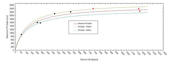
Let us imagine that a user has the results of inspection of the pipeline for the first 1,5 years after the beginning of the exploitation but he wants to predict corrosion damage (maximum cavity depth) for the next 1.5 year. Figure 5 shows that the output plot of OLI software (solid lines) yields the acceptable agreement with future inspections (red circles). Let us also imagine that the user also wants to estimate the integrity of pipeline (probability of failure) for 5 years after beginning of the exploitation. Figure 6 shows this probability (the probability that the depth of the deepest cavity increases the wall thickness).
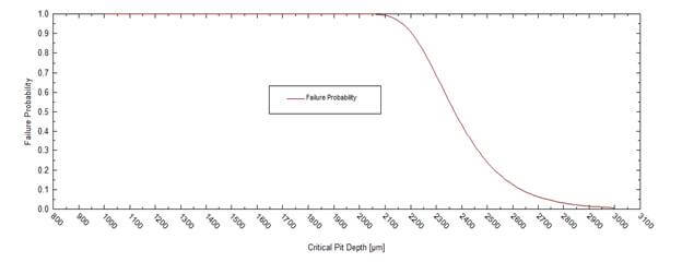
By using Figure 5 the user (who knows the thickness of pipeline’s wall) can estimate the integrity of the pipeline for t = 5 years. (Practically all pipelines have wall thickness d ≥ 0.1 in = 2540 μm.)
To speak to an OLI technical or sales specialist please register your interest here https://www.olisystems.com/contact-us
References
- M. Kowaka, H. Tsuge, M. Akashi, K. Masamura; H. Ishimoto. Introduction to Life Prediction of Industrial Plant Materials: Application of the Extreme Value Statistical Method for Corrosion Analysis. Allerton Press, 1994.
- D. D. Macdonald and G. R. Engelhardt, Predictive Modeling of Corrosion. In: Richardson J A, et al. (eds.) Shrier’s Corrosion, 2, pp. 1630-1679 (2010).
- P. M. Aziz, Application of the Statistical Theory of Extreme Values To the Analysis of Maximum Pit Depth Data for Aluminum, CORROSION. 1956;12(10):35-46.
- Zikerman, “Diagnosis of Corrosion in Pipelines”, Nedra, Moscow, 1972.
- Engelhardt, and D. D. Macdonald. “Unification of the Deterministic and Statistical Approaches for Predicting localized Corrosion Damage. I Theoretical Foundation”, Corros. Sci., 46, pp. 2755-2780 (2004).
- J. Laycock; R. A. Cottis, P.A. Scarf, Extrapolation of Extreme Pit Depths in Space and Time, J. Electrochem. Soc., 137 (1990) 64 -69.