


Engineering decisions frequently involve trade-offs among costs and benefits that occur at different times. The practical science of engineering economics was originally developed to deal with determining the best alternative given many options, considering the costs and benefits of each option. Engineering project investments are typically classified as capital investments (i.e., fixed capital cost and working capital cost) or operating expenses (i.e., direct production costs, fixed costs, and plant overheads). Engineers must be able to make the optimal choice among several technically feasible alternatives. Engineering Economics is the science that deals with quantitative analysis techniques used to select a preferred alternative from several technically viable ones.
However, regardless of the technical option selected, the manufacturing processes must be economically profitable to make it commercially sustainable. In other words, the manufacturing cost must be less than the income generated through product sales. Process optimization, therefore, requires the capability to analyze the influence of processing techniques, sequencing, equipment design, and operating parameters on the economic performance.
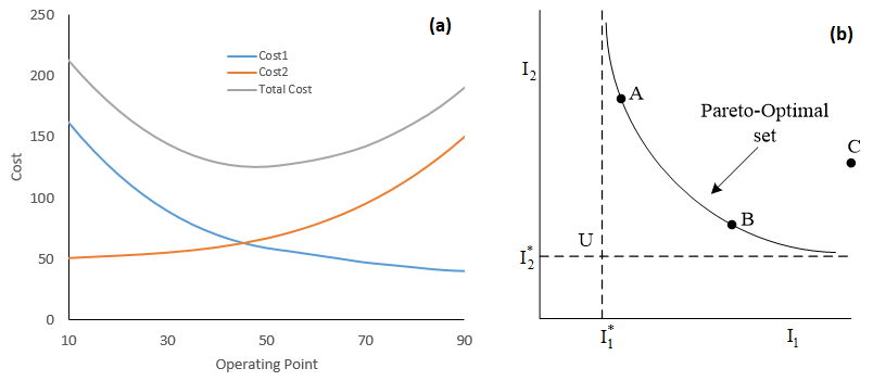
Single-objective optimization often deals with maximizing profit or minimizing cost in a process. The idea is to find a global optimum solution (Figure 1a) within the operating bounds or constraints.
However, in real chemical processes, it is not uncommon to have two or more objectives that should be optimized at the same time, moreover, the objectives could be conflicting in nature. It is worth noting that the principle of multi-objective optimization with conflicting objectives is conceptually different from that of single-objective optimization. Solution of multi-objective optimization problems give an entire set of equally good solutions known as Pareto-optimal set (Figure 1b). There may not be a solution which is better than any other solution on the set (A and B both are acceptable, but not C) with respect to all the objectives (I1 and I2 are objectives). The entire set could be an acceptable solution, and the choice of one solution over others require additional information and rationale on the system.
The OLI software platform provides unique data properties and simulation software innovations to tackle complex water chemistry-based operational challenges in oil & gas, water treatment, mining, power generation and chemicals industries. The OLI software platform also provides an excellent foundation to deliver flowsheet model optimization to optimize chemical processes.
As part of the new V11 release, OLI Systems has developed a general-purpose optimization capability, the OLI Optimizer Tool, for its process flow sheeting software, OLI Flowsheet: ESP. The OLI Optimizer tool enables optimization of process parameters (stream and block parameters), thermodynamic parameters (interaction parameters, equilibrium K), kinetic parameters (standard and user-defined), and user-defined calculator options (executed at run-time). Table 1 provides the scope of optimization in OL Flowsheet: ESP.
Table 1: Optimization scope in OL Flowsheet: ESP in V11
| Optimization scope | Type | Description |
| Process variables
|
Stream parameters | Any stream input parameters |
| Block parameters | Any block input parameters | |
| Thermodynamic parameters | UNIQUAC interactions | UNIQUAC, extended UNIQUAC and pressure dependent UNIQUAC |
| Midrange interactions | Midrange and pressure dependent midrange | |
| SRK interactions | Mixing rule parameters, Kabadi-Danner coefficient¥ | |
| Kfit coefficients | Temperature and pressure dependent parameters | |
| Pitzer interaction¥ | Ion-molecule, molecule-molecule interaction | |
| Bromley interaction¥ | Ion-ion interaction | |
| Kinetic parameters | Std or Arrhenius | Arrhenius rate equation |
| User-defined | User defined rate equation | |
| Calculator block | User-defined | User defined calculation over the flowsheet |
| ¥ for AQ framework only or not used in MSE framework | ||
In a previous post we demonstrated a few examples where process variables (parameters for streams and unit operations/blocks), kinetic parameters and some thermodynamic parameters of OLI’s MSE and Aqueous framework were optimized. In this simple example, we place particular focus on improving process economics.
Natural gas is predominantly methane, however, the side-products of processing natural gas are lighter components, e.g., ethane (C2), propane (C3), butanes (C4), pentanes (C5), to heavier hydrocarbons, hydrogen sulfide (H2Swhich is usually converted to elemental sulphur), carbon dioxide (CO2), helium (He) and nitrogen (N2). Natural gas liquids (NGL), namely liquefied petroleum gas, (LPG) consisting mainly of propane and butane, gasoline consisting mainly of pentane, solvent oil consisting mainly of hexane and heavier hydrocarbons are recovered through turboexpander technology. The LPG recovery unit plays a vital role in boosting revenue by increasing liquids recovery from the feed natural gas. Turboexpander technology with an absorber column is conventionally used for >99% propane recovery in many natural gas processing plants.
Table 2: Feed natural gas composition
| Temperature (°C) | 30 | ||||
| Pressure (kPa) | 5000 | ||||
| Total Flow (kgmol/hr) | 2988 | ||||
| Inflows (mole %) | |||||
| C3H8 | 1.48 | ||||
| C4H10 | 0.2 | ||||
| C5H12 | 0.06 | ||||
| C6H14 | 0.03 | ||||
| CH4 | 91.22 | ||||
| CO2 | 0.2 | ||||
| C2H6 | 4.96 | ||||
| IPENTAN | 0.1 | ||||
| ISOBUTANE | 0.26 | ||||
| N2 | 1.49 |
In turboexpander technology, an expander reduces the pressure of the inlet gas, and produces a cryogenic temperature, which aids the recovery of NGL and LPG from the feed gas stream. Table 2 lists the composition of feed natural gas. A process flowsheet model was created using OL Flowsheet: ESP and Figure 2 describes the process flow diagram.
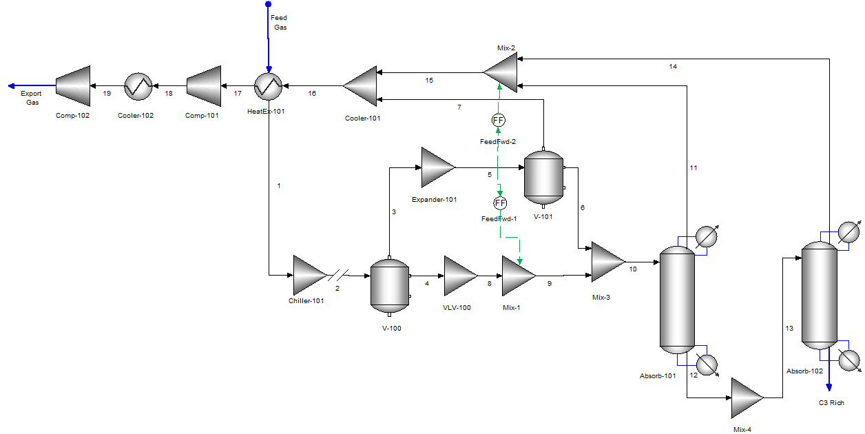
The feed gas stream exchanges heat with other utility streams in the process to recover waste heat in the process. After the heat exchange (HeatEx-101), the feed gas stream is being cooled in a chiller (Chiller-101) which is through liquefaction of refrigeration cycle. The heavy hydrocarbons condense as liquid, and the light ends (lighter hydrocarbon) form a vapor stream from the two-phase separator (V-100), which is routed to an expander (Expander-101). The turboexpander expands the vapors and produces cryogenic temperature. This unit adds refrigeration to the overall system, which boosts LPG recovery. After expansion, a two-phase separator (V-101) routes the lighter hydrocarbons to the export or residual gas line and heavier hydrocarbons to the absorption tower (Absorb-101). The absorption tower removes remaining lighter hydrocarbons from the top of the tower and enriches the bottom stream with C3+ components. The bottom product from Absorb-101 is routed to Absorb-102 which acts as a deethanizer tower. In Absorb-102, C2- components are removed from the top of the tower and bottom product is further enriched in C3+ components.
In LPG recovery process, liquid from the deethanizer bottom containing C3+ content is then routed to a debutanizer tower (not modeled here). LPG is recovered from the debutanizer tower as top product, whereas NGL is recovered from the bottom. The residue gas with mostly lighter hydrocarbons, e.g., mainly methane is compressed in gas compressors (Comp-101, Comp-102) and delivered into a natural gas pipeline grid or customer pipeline.
There are a few challenges in the LPG recovery process. A suboptimal operation in any of the following: the chiller, a low-temperature separator, turboexpander, absorbers reboiler/condenser may overburden the recovery process and reduce profit. Propane slippage with vapor stream may reduce LPG recovery. Moreover, compressing cost for the residual gas needs to be low for the process to be optimum which is tied with the turboexpander operation. Thus, an optimization problem can be formulated for maximizing profit where chiller exit temperatures and turboexpander exit pressures are independent variables. The profit is defined in the objective function, and chiller exit temperatures and turboexpander exit pressures are defined as decision variables.
Profit = [Revenue form sales (C3 Rich stream) – Compression cost (Comp 101, Comp 102) – Cooling cost (Chiller-101, Cooler-101, Cooler-102)]
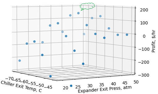
Decision variables are chiller exit temperatures (maximum bound: -45C, minimum bound: -65C) and turboexpander exit pressures (maximum bound: 50 atm, minimum bound: 19 atm). Few others optimization convergence parameters are kept as default. For simplicity, let us assume the C3+ has a price of $0.2/kg and power consumption cost is $0.05/kWh. Optimizer converged to a solution after 14 optimizer iterations with chiller exit temperature and turboexpander exit temperature and pressure of -61.8C and 41.5 atm, respectively. Figure 3 represents the optimizer state at each iteration. Figure 4 represents optimizer calculation results which includes snapshot of objective functions definition, initial and final state of variables and convergence details.

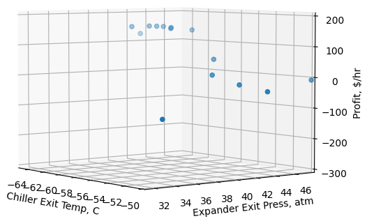
To ensure the solution is not a local minimum/maximum within the bounds, and to verify that an optimal solution is being achieved, we conducted a sensitivity analysis of chiller exit temperatures and turboexpander exit pressures on profit. Figure 5 represents the sensitivity analysis on profit. The figure shows highest and lowest gross profit in the operating conditions region. It is clear that an optimal solution exists within the bounds (green cloud callout pointing around the maximum) and the tool finds the global maximum within the bounds.
It is to be emphasized that there are varieties of optimization problems that could be formulated and studied based on process knowledge, and a simple example is presented here to illustrate the concepts, techniques, and interpretation of results. Either a global solution or set of pareto optimal solutions (no solution is considered superior to others with respect to all objective functions), the choice of one solution over the others require additional knowledge of the problem, and often this knowledge is intuitive and non-quantifiable. Optimization is very useful to process designers, operators, and decision makers since it narrows down the choices from larger number of possibilities and helps them selecting a preferable operating point (preferred solution) or profitable solution from among the set of many acceptable operating and/or design conditions.
Please tune in for more interesting applications which will be presented in upcoming articles. OLI Systems would like to work with clients in optimizing their flowsheet applications and our experienced team of Application Engineers and Consultants will be glad to discuss this further.
OLI Systems offers a unique combination of material properties, models and software that uses first principles based thermodynamic and electrochemical modeling. The OLI property database of over 6,000 species covers over 80 elements of the periodic table. OLI’s physical property methods, and property parameters and data are the ideal choice to suit your simulation needs. OLI Systems has expert scientists, thermodynamicists, engineers and consultants ready to help with thermodynamic data development, complex chemistry definition, sponsored-research projects and Joint Industry Programs (JIPs) for industrial water and electrolyte chemistry applications.
In addition to the OLI Optimizer tool and updates the OLI Windows software (OLI Studio, OLI Flowsheet: ESP, OLI Alliance Engine and OLI Engine: Developer Edition), the V11 release also includes a brand-new OLI Cloud platform to fuel the industrial digital transformation. You can learn more about the OLI Cloud Platform here.
Contact OLI for more information or to schedule a meeting with an OLI expert.


