


Generally speaking, there are two different ways of defining corrosion damage [1]. From a so-called “scientific” point of view, the critical parameters (corrosion potential, chloride content, etc.) can be defined as the parameters required for depassivation of the metals, whereas from a practical, so-called “engineering” point of view, corrosion damage is usually associated with visible or “acceptable” deterioration of the metallic structure. These definitions have different time scales. Thus “scientific definition” is related to the initiation stage of degradation whereas the “engineering” definition is related to the visible or acceptable stage of corrosion.
In the case of localized corrosion for describing corrosion damage from the “engineering” point of view, very often, it is sufficient to obtain information about only the deepest corrosion event (pit, crack), because failure in the system commonly occurs when the depth of the deepest corrosion event amax exceeds some critical value, acr. Usually, acr is the thickness of the wall of a pipe, for example, or the depth of a pit transitioning into an unstable crack [2].
Estimating amax as a function of time and for a given set of mechanical and environmental conditions usually represents a complicated task connected with mass and charge transport problems. There is no possibility to directly predict amax (t) by using OLI software. (Up to now, there is only a possibility to predict amax (t) in large systems when the dependence amax (t) ) in the series of small systems (coupons) is known by using the extreme value statistics module in OLI’s software.)
However, OLI’s software can be used for the prediction of initiation of localized corrosion, i.e. for the prediction of corrosion damage from the “scientific” point of view. This is evident in the case of pitting corrosion because OLI’s software can be used for predicting the repassivation potential, Erp, in rather complicated electrochemical systems. Thus, if the repassivation potential of the systems is larger than the corrosion potential for the same system, Ecorr, the incubation of pits (incubation of pitting corrosion) becomes impossible by definition. The scientific bases that are used for estimating Erp and Ecorr in OLI’s software can be found in Ref. 3.
The same is true in the cases of environmental stress corrosion cracking (SCC) and corrosion fatigue (CF). In reality, regarding the transition of a pit into a crack, it is assumed that a pit immediately transforms into a crack if its depth exceeds some critical value atr. As of now, the most widely accepted set of criteria for the transition of a pit into a crack is the Kondo criteria [4]. According to these criteria, two conditions must be satisfied for crack nucleation to take place from a pit, namely,
KI >KISCC for SCC or ΔK > ΔKth (for CF) (1)
and
Vcrack >Vpit (2)
Here, KI and KISCC are the stress intensity factor and critical stress intensity factor for the propagation of a stress corrosion crack, respectively; △K is the stress intensity factor range, and △Kth is the threshold stress intensity factor range for fatigue crack propagation, respectively. The first requirement defines the mechanical (fracture mechanics) condition that must be met for the prevailing stress and geometry, while the second simply says that the nucleating crack must be able to ‘outrun’ the pit. (See an example of stress corrosion cracking in Figure 1.)
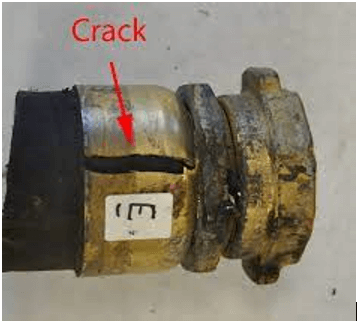
Figure 1. A real example of stress corrosion cracking.
In general case KI and △K → 0 at a→0 regardless of the applied stress, σ, and stress intensity factor, Δσ. Thus, for example, in the simplest case . Accordingly, it is evident that if Erp > Ecorr corrosion pit was not nucleated, and neither SCC nor CF also cannot be nucleated.
Similar to pitting corrosion, crevice corrosion (CC) is initiated with the breakdown of stainless steel’s protective oxide film and continues with the formation of shallow pits. However, rather than occurring in plain sight, crevice corrosion—as its name implies—occurs in crevices. It must also be noted that applying OLI’s software for predicting the possibility of pit initiation inside the crevice requires knowledge of the chemical composition of the solution inside the crevice that can be substantially different from the bulk composition.
It must be also mentioned that sometimes hydrogen embrittlement (HE) initiates inside pits due to the substantial accumulation of hydrogen on the bottom of pits. In some cases, pitting corrosion not only initiates SCC in the alloy, but it also induces hydrogen entry into the alloy leading to HE.
Examples of the estimation of the probability of the initiations of localized corrosion
The condition
Erp > E (3)
where E is the metal potential (E = Ecorr in the case of free corrosion) can be considered to be sufficient for preventing pitting corrosion and accordingly for preventing localized corrosion in the ‘scientific’ sense in the form of pitting corrosion, SCC, CF, and in some cases in the form of crevice corrosion and HE. But Condition (3) cannot be considered to be necessary for preventing localized corrosion damage in the ‘engineering’ sense. Thus, for example, it can occur that the depth of the deepest pit cannot reach the critical dimension, acr, during the observation time, t.
It is well known that chloride ions can often be the main factor for initiating pitting corrosion. Particularly, chloride-induced pitting corrosion is a known issue with austenitic stainless steel alloys such as 304 and 316. Accordingly, here we begin from the simplest example – corrosion of Alloy 316 in aerated full agitation solution with the presence of NaCl (see Figure 2). The temperature in all the examples considered below is chosen to be 25 0C.
As we can see, at [NaCl] < [NaCl]cr ≈ 0.0086 m Condition (3) holds, and Alloy 316 can be considered to be immune for the pitting corrosion (and accordingly to SCC and CF). But, at [NaCl] >[NaCl]cr localized corrosion can occur. Accordingly, we can expect that stainless steel 316 will be susceptible to localized corrosion in the aerated seawater.
Calculations show that in the case of Alloy 304 [NaCl]cr ≈ 0.0019 m. It means that Alloy 316 is somewhat more resistant to the initiation of chloride-induced pitting than Alloy 304 (a fact mentioned in the literature). Calculations also show that both alloys (304 and 314) are resistant to chloride-induced pitting corrosion in deaerator solutions.
Below calculations were performed for the corrosion of Alloy 316 in the typical (artificial) seawater with the following chemical composition: NaCl 0.47 m, CaCl2 m, CaO 3.75×10⁻³m, MgCl2 0.0291 m, MgSO4 0.0244 m, SO3 4.22×10⁻³, CaCO3 2.49×10⁻³ m.
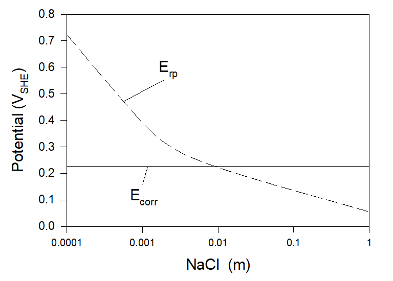
Figure 2. Corrosion and repassivation potentials at the corrosion of Alloy 316 in full agitation NaCl aerated solution at T = 25 0C.
Figures 3 and 4 show polarization curves for the case of corrosion of Alloy 316 in aerated artificial seawater under static and full agitation hydrodynamic conditions at T = 25 0C. As we can see neither corrosion potential nor repassivation potential practically do not depend on hydrodynamic conditions. Particularly, Ecorr ≈ 0.2285 VSHE and Erp ≈ 0.0740 VSHE.
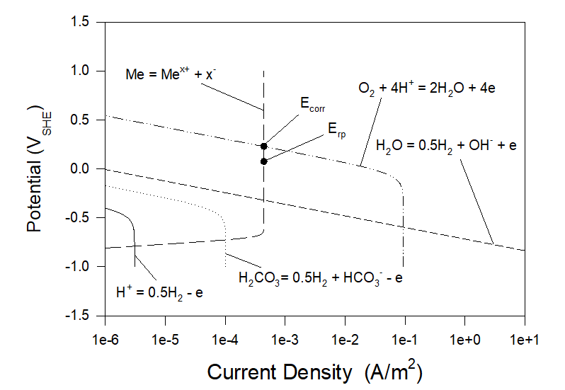
Figure 3. Polarization curves for the case of corrosion of Alloy 316 in aerated artificial seawater under static hydrodynamic conditions at T = 25 0C.
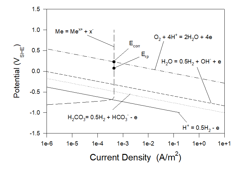
Figure 4. Polarization curves for the case of corrosion of Alloy 316 in aerated artificial seawater under full agitation hydrodynamic conditions at T = 25 0C.
As we can see the incubation of localized corrosion (corrosion in “scientific” sense) is inevitable in the case of Alloy 316 in seawater. The question arises what can be done to definitely prevent localized corrosion in this case? It can be suggested two methods to fulfill this task.
The first method is the addition of inhibitors of localized corrosion (for example NO3–) into the solution. Thus Figure 5 yields calculated values of repassivation and corrosion potentials as functions of the NaNO3 concentration added to the artificial seawater. Calculations show that at [NaNO3] > [NaNO3]cr ≈ 0.20 m Condition (3) is fulfilled and, accordingly, localized corrosion cannot occur. In such a manner OLI’s software can be used to find the minimum amount of inhibitors required to protect the system from localized corrosion and by doing so to reduce the expenses connected with the application of inhibitors.
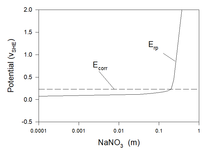
Figure 5. Corrosion and repassivation potentials at the corrosion of Alloy 316 in aerated artificial seawater with the addition of sodium nitrate at T = 25 0C.
It must be noted that practical employment of this method can be rather complicated in the general case. Thus, it is unclear how this method can be applied in the case of external corrosion of the metal construction in the open sea.
The second method for preventing localized corrosion is the so-called cathodic protection method or more precisely impressed current cathodic protection (ICCP) method. ICCP systems consist of permanent inert anodes, such as mixed metal oxide (MMO) coated titanium and ribbon, conductive ceramics or conductive coatings and an external DC power source to supply sufficient current to the steel to overcome the natural corrosion activity (see Figure 6.)
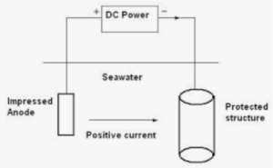
Figure 6. Scheme of the ICCP method.
Let us consider the case shown in Figure 4. Let us also imagine that by using DC Power we keep the potential of the metal, for example, equal to 0.05 VSHE which is less than the repassivation potential of 0.074 VSHE (see Condition (3)). It means that at this potential (0.05 VSHE) the system will be immune to localized corrosion. By using the OLI software we can obtain the following information (see Figure 4), The general corrosion current density is very low (4.45×10⁻⁴ A/m2 and does not change. The net current density becomes negative (the metal becomes a cathode) and low (0.014 A/m2). It means that the energy consumption by the DC power will be also low. The cathodic current densities connected with the hydrogen evolution reactions H+ = 0.5H2 -e, H2CO3 = 0.5H2 + HCO3– – e, H2O = 0.5H2 + OH– – e are extremely low (2.79×10⁻¹⁰ A/m2, 1.32×10⁻⁸ A/m2 and 3.33×10-70 A/m2 correspondingly). Accordingly, hydrogen embrittlement in this system is extremely unlikely.
It must be noted that impressed current cathodic protection can often result in hydrogen embrittlement, which can cause trouble with high-strength steels [6]. Therefore, the limiting potential for hydrogen embrittlement should be examined in detail as a function of the cathodic protection potential. Thus, it is clear that the higher the applied potential of the metal, E, (or the less the difference Erp – E) the less will be the probability of hydrogen embrittlement.
Conclusion
OLI software yields a reliable and convenient tool for predicting pitting corrosion. In the case when pitting corrosion is unlikely it is also unlikely that other forms of localized corrosion (SCC, CF, etc) that can be nucleated from the growing pits.
In the case when Erp is less than Ecorr pitting corrosion can take place. In order to prevent pitting corrosion, it is possible to increase Erp to be above Ecorr by adding inhibitor ions (for example, NO3–) to the solution or to reduce metal potential, E, below Erp by using an external amplifier (ICCP method).
In both cases, OLI’s software offers unique possibility for optimizing methods for preventing localized corrosion.
In the first case, OLI’s software yields the possibility to find the minimum amount of inhibitors required to protect the system from localized corrosion and by doing so to reduce the expenses connected with the application of inhibitors.
In the second case the metal potential, E, is reduced below Erp by using the external amplifier. In this case, OLI’s software yields the possibility to estimate the minimum of the difference Erp – E to minimize energy consumption and to reduce the possibility of hydrogen embrittlement.
References
- Angst, B. Elsener, C.K. Larsen, Ø. Vennesland, Critical chloride content in reinforced concrete – A review, Cem. Concr. Res. 39 (2009) 1122–1138.
- D. Macdonald and G. R. Engelhardt, 2010 Predictive Modeling of Corrosion. In: Richardson J A et al. (eds.), Shreir’s Corrosion, 2, pp. 1630-1679 Amsterdam: Elsevier.
- Anderko, 2010 Modeling of Aqueous Corrosion. In: Richardson J A et al. (eds.), Shreir’s Corrosion, 2, pp. 1585-1629 Amsterdam: Elsevier
- Kondo, Prediction of Fatigue Crack Initiation Life Based on Pit Growth, Corrosion 1989, 45, 7–11.
- B. Kannan and W. Dietzel, Pitting -induced hydrogen embrittlement of magnesium-aluminum alloys, Material and Design, 42, (2012) 321-320.
- Pederferri, Cathodic protection and cathodic prevention, Construction and Building Materials, 10, pp.391-402, 1996.