


In any operation, cost lies at the forefront of decision-making; it is often the dividing line between stop and go. The story is no different in chemical process settings, where cost works in concert with chemistry to strike a balance of acceptable level of risk. In this blog, we will walk through a cooling tower case study to demonstrate how to employ the OLI Process API to predict key process impacts and, by extension, high-level financial outcomes.
Typical Use-Case of Process API
In a recent piece, we learn that the OLI Process API is the Cloud equivalent to the OLI Flowsheet: ESP desktop product. The latter is a process simulator that leverages the extensive OLI electrolytes database, and can model phenomena such as crystallization, ion exchange, or solvent extraction, and predict stream parameters such as thermodynamic properties, chemical speciation, pH, and scaling tendencies.
After a process is designed in Flowsheet: ESP, it is uploaded to the OLI Cloud. From here, a Python script is constructed to read in and store all the baseline model properties into a file. Next, the script reads in a set of user data, from which relevant parameters are extracted and substituted into the model as inputs. This is done to evaluate how the manipulated parameters affect the system outputs.
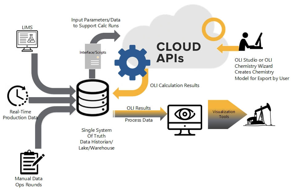
Figure 1. Graphic of workflow for leveraging OLI’s Cloud solutions.
First, the user uploads their Flowsheet to the OLI Cloud. Next, a script reads in system data, extracts relevant parameters, and uses these values as inputs to the Flowsheet. The model calculations run inside the Cloud, and outputs are sent back to the user.
Applying Economics in Post-Processing
After each run of the model with Process API, the outputs are stored in a system of the user’s choice, allowing full flexibility in data post-processing and analysis. To evaluate the economic implications of the manipulated input parameters, we can follow the workflow below:
- Execute automated runs of the model via Process API, whereby one input is changed at a time.
- For example, run a cooling tower model with inlet air temperature of 25-60C at increments of 5 Next, run the model at different inlet air relative humidities.
- Isolate the model outputs that have financial bearing on the system; for a cooling tower, this could be makeup water and blowdown flowrates.
- Multiply each of these outputs by the associated cost (e.g. $/m3).
- Plot the data to visualize how the modulated input affects the system costs.
- Economic information can be plotted in tandem with other outputs such as scaling tendencies. This can facilitate a cost-benefit analysis.
Cooling Tower Case Study
To exemplify this capability, we used a generic cooling tower Flowsheet model shown in Figure 2. In optimizing a cooling tower system, the aim is to maximize the number of process cycles by minimizing blowdown and makeup water, while mitigating the risk for scaling. Ultimately, the system must still meet the water temperature specifications required for the process. In the model below, the inlet air stream mimics ambient conditions in its composition and temperature. The heat exchanger labeled “Process” represents the expenditure of cooled water in heat exchangers elsewhere in the plant.
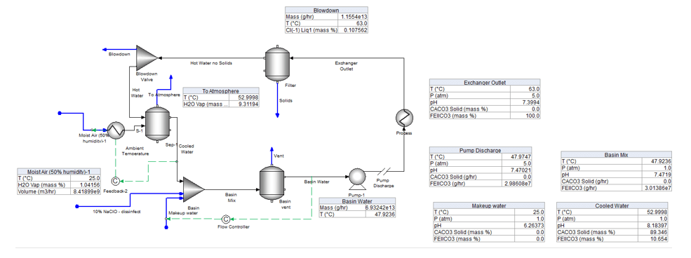
Figure 2. Flowsheet model of a generic cooling tower system.
After uploading the Flowsheet to the Cloud, we generated a dataset to read in as changing inputs to the model; these modulated parameters are listed in Table 1.
Table 1. List of adjusted input parameters.
| Adjusted Input Parameter | Application to a Real Cooling Tower |
| Blowdown Valve Outlet Split | Blowdown Flowrate |
| Inlet Air Temperature | Ambient Air Temperature |
| Inlet Air H2O Mole Fraction | Ambient Air Humidity |
| Flow Controller Target Value | Basin Water Flow |
In the post-processing step, we multiplied the volumes of makeup water and blowdown (m3/hr) by the corresponding estimated cost outlined in Table 2 (1-3). It is important to note that water usage costs vary widely by location; for instance, disposal at some sites may require additional transportation.
Table 2. Water usage and associated cost per unit volume, approximated based on References (1-3).
| Water Usage | |
| Makeup Water Supply | $0.50/m3 (1-2) |
| Blowdown Disposal | $15/m3 (1,3) |
With the OLI Process API and subsequent output data analysis, we arrived at the sensitivity plots displayed in Figure 3. These plots demonstrate the effect of each isolated parameter on estimated water usage costs. As an example of preliminary cost-benefit analysis, in each scenario, we have included the predicted amounts of mineral scale in the return water (stream labeled “Hot Water” in Figure 2)
Sensitivity Analyses
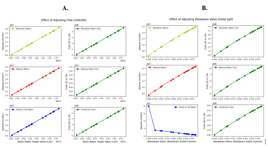
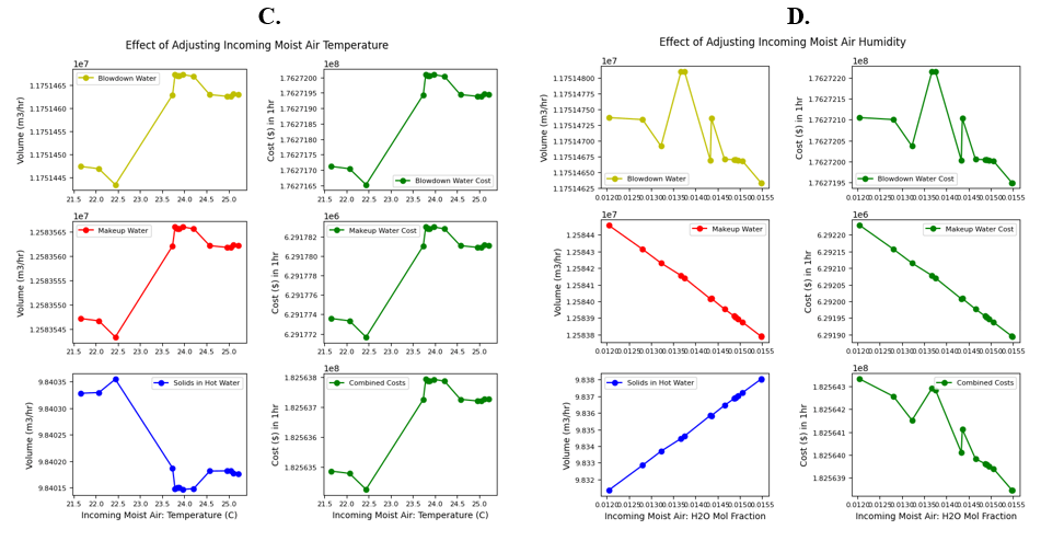
Figure 3. Collection of sensitivity analysis plots.
A) Effect of adjusting flow controller’s target value of basin water total flow. B) Effect of adjusting the blowdown valve outlet fraction split for blowdown. C) Effect of adjusting inlet air temperature (°C). D) Effect of adjusting inlet air relative humidity.
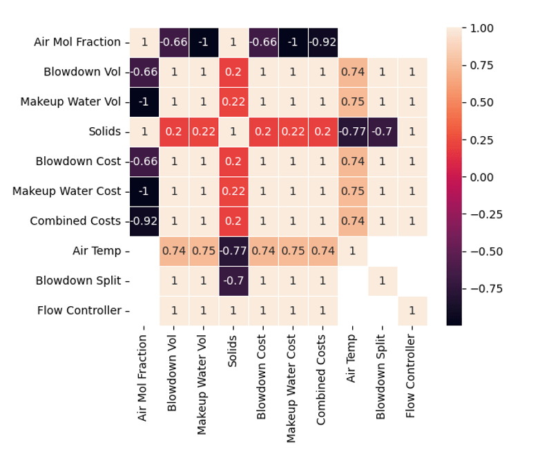
From the sensitivity analyses, we extracted the correlation matrix in Figure 4, where each cell quantifies the relative relationship between two isolated parameters (4-5). For example, the correlation between “Flow Controller” and “Makeup Water Cost” shows a value of exactly 1, indicating a directly proportional relationship between basin water flow and fresh water expenses (4–5). On the other hand, the correlation between “Air Temperature” and “Solids” at -0.77 indicates that these two parameters are inversely related (4–5). The more extreme a value (i.e. the closer to 1 or -1), the stronger the correlation (4-5). The blank cells correspond to different input pairs, which were not analyzed for correlation.
(4). The label “Solids” refers to mineral scaling in the return water.
Conclusions and Looking Ahead
In this blog, we demonstrated how to leverage the OLI Process API to manipulate certain inputs of interest, enabling us to analyze potential economic impacts based on water usage. In tandem with water usage, we can conduct a more comprehensive cost-benefit analysis that optimizes overall process cost and scaling tendencies. In future renditions, this approach can be coupled with the OLI Corrosion Analyzer to optimize cost while minimizing predicted corrosion rates. Similar to the work presented in Bueso et al., looking ahead, we can conduct a more rigorous optimization by coupling OLI’s electrolytes database with a neural network ML model (4). With this approach, we can maximize water reuse based on the combined effects of brine chemistry and process conditions in a variety of water treatment systems (4). This framework is applicable to other industries and opens the door for exciting user-specific analyses. To learn more about how this can be leveraged for your system, contact OLI.
References
- Saltworks Technologies. Frac & Shale Produced Water Management, Treatment Costs &
Options. June 14, 2018. https://www.saltworkstech.com/articles/frac-shale-produced-water-management-treatment-costs-and-options/ (accessed 2024-03-07).
- McIntyre, J. P. Industrial Water Reuse and Wastewater Minimization. General Electric Company,
Water & Process Technologies, 2006. https://www.waterprofessionals.com/wp-content/uploads/industrial_water_reuse.pdf (accessed 2024-03-07).
- OGAP 2007 Produced Water Factsheet: Options and Costs for Disposal of Produced Water; Oil
and Gas Accountability Project of EARTHWORKS: Durango, CO, 2007. https://earthworks.org/wp-content/uploads/2021/09/MicrosoftwordProducedWaterFactsheet2.pdf (accessed 2024-03-07).
- Bueso, M. C.; de Nicolás, A. P.; Vera-García, F.; Molina-García, Á. Cooling tower modeling
based on machine learning approaches: Application to Zero Liquid Discharge in desalination processes. Applied Thermal Engineering 2024, 242, 122522. DOI: 10.1016/j.applthermaleng.2024.122522
- Brydon, M. Correlation and Scatterplots. Basic Analytics in Python, Simon Fraser University,
- https://www.sfu.ca/~mjbrydon/tutorials/BAinPy/08_correlation.html (accessed 2024-03-07).