


 Corrosion issues in chemical processes
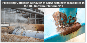
Chemical process environments often contain corrosive multicomponent systems including acids, salts and their mixtures accompanied by various types of gases. These components potentially lead to significant corrosion issues in chemical processes brining about equipment failure and the regular shutdowns and overhauls of the chemical plants. For instance, high corrosion rates can be seen on piping, pumps, boilers, and reactors depending on the operational conditions. A comprehensive study by National Association of Corrosion Engineers (NACE) in 2016 showed that the direct cost of corrosion in industry is B$276 / year which is equivalent to 3.1% of US GDP.
Why develop theoretical corrosion models?
In order to prevent corrosion problems, selection of appropriate corrosion-resistant alloys (CRAs) is usually guided by their reported corrosion rates and applicability domains at specific operating conditions. However, this information is rarely available for corrosion in multi-component systems at varying fluid compositions or acid gas partial pressures, especially at higher temperatures. Production from deep wells in upstream oil and gas operations, organic/inorganic acids production processes, and power plants environments are examples of such systems. Localized and general corrosion of CRAs can be evaluated by analyzing electrochemical characteristics of the alloys, including the corrosion potential (Ecorr), repassivation potential (Erp), and depassivation pH (pHd). In particular, Ecorr and Erp can be used together to predict the onset of localized corrosion and to estimate its propagation rate for different types of CRAs. However, the electrochemical parameters such as Ecorr or Erp are usually obtained from laboratory tests in relatively simple corrosive environments and are not available at complex operational conditions. Therefore, there is a need to establish predictive models that could quantify the behavior of CRAs in complex process environments. This need has motivated the development of practical models that not only explain the corrosion mechanisms but also simulate the effects of environmental parameters on the corrosion properties of CRAs in complex environments.
Key parts of the OLI Corrosion model
The key parts of the OLI Corrosion model available in OLI Platform V11 can be summarized as below:
- Computation of the thermodynamic properties of the aqueous environment in the bulk and at the surface constitutes the foundation of the model. For this purpose, an aqueous thermodynamic model is used to predict the properties of the system at equilibrium including the speciation, activity of species and other thermophysical and transport properties.
- Alloy dissolution in the active state is modeled by the Butler-Volmer equation, which takes into account the adsorption of electrochemically active species and their surface coverage to calculate the metal dissolution current density.
- The active-passive transition and, consequently, the total anodic dissolution current (i.e., the active dissolution and passive dissolution) are expressed by solving an equation that considers the change of the passive layer coverage fraction with time in the steady-state limit.
- The repassivation potential is calculated by solving, in the limit of repassivation, the expression for the current density in an occluded localized corrosion environment. This expression takes into account the effects of competitive adsorption of active species (such as Cl– and H2S) on anodic dissolution. Adsorption of various aggressive species (e.g., Cl–) and inhibitive species (e.g., NO3– or SO42-) has an effect on alloy dissolution and the formation of metal oxide (or sulfide) layer, which are modeled to accompany the repassivation process.
By combining steps I through III as described above, the corrosion potential (Ecorr) and the general corrosion rate are computed by calculating a synthesized polarization curve based on the mixed-potential theory. Taking into account that localized corrosion cannot occur at potentials below the repassivation potential, the calculated Erp value (resulting from step IV) is then compared with the Ecorr value to predict the occurrence of localized corrosion and to estimate the maximum propagation rate of localized corrosion as a function of environmental conditions.
What alloys and environments have been studied in this article?
OLI Platform V11 is capable of predicting corrosion behavior of various types of alloys including, but not limited to, nickel-base alloys and stainless steels. Table 1 shows the chemical composition of the alloys studied in this article which represent two types of nickel-base alloys with different Cr and Mo contents as well as a martensitic stainless steel. The performance of the model has been verified in various classes of environments, i.e., (a) single acids, (b) mixed acids, and (c) brines with or without oxidizing agents.
Table 1. Nominal compositions of the alloys studied in this article (weight percent)
| UNS No. | Common name | Ni | Fe | Cr | Mo | C (max) | W | Other(wt% max>1) |
| N06022 | 22 | Bal. | 3.0 | 22 | 13.0 | 0.015 | 3.0 | Co 2.5 |
| N10276 | 276 | Bal. | 5.5 | 16.0 | 16.0 | 0.01 | 4.0 | Co 2.5 |
| S41425 | S13Cr | 5.9 | Bal. | 12.1 | 1.9 | 0.03 | 0.0 |
Single and mixed acids
The main advantage of a mechanistic model is being able to predict the behavior of alloys in multicomponent mixtures using parameters generated from simpler, building-block systems. In the case of acids, we reproduce the corrosion behavior of alloys in individual acids by adjusting the relevant model parameters. Then, we apply the model to predict the corrosion behavior in mixed acids. Here, we analyze the behavior of UNS N06022 in mixtures of hydrochloric and nitric acids.
First, the available experimental corrosion rate data in single-acid, HCl and HNO3 solutions have been used to develop the relevant model parameters. Figures 1 and 2 show the calculated and experimental corrosion rates for UNS N06022 in HCl and HNO3 solutions, respectively. Corrosion in these acids proceeds according to different mechanisms. HCl is a non-oxidizing acid, in which the chloride ions (Cl–) have a considerable effect on the active-passive transition. On the other hand, HNO3 is an oxidizing acid, in which the corrosion potential is elevated due to a strong additional cathodic reaction of HNO3 reduction. In single-acid HCl solutions, anodic dissolution is in the active state whereas the presence of HNO3 leads to the passive dissolution of the metal.
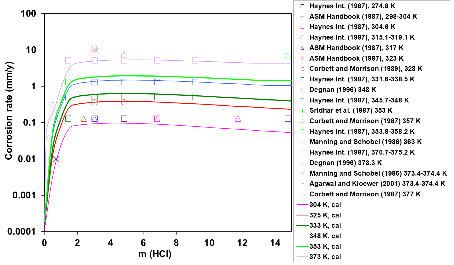 Figure 1: Calculated (lines) and experimental (symbols) corrosion rates of UNS N06022 in HCl aqueous environments at temperatures ranging from 304 to 373 K.
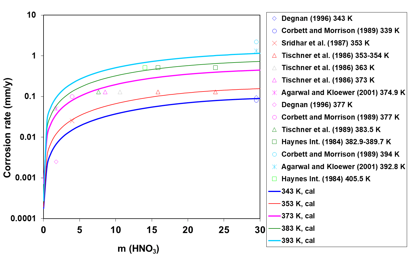 Figure 2: Calculated (lines) and experimental (symbols) corrosion rates of UNS N06022 in HNO3 solutions at temperatures from 343 to 393 K.
In HCl + HNO3 mixtures, both the acidity and the electrochemically active Cl– and NO3– ions have a substantial impact on the active-passive transition. Therefore, the corrosion rate patterns in mixed acids are not a simple average of those in single acids solutions. Figure 3 shows the calculated and experimental corrosion rates for UNS N06022 in mixed HCl + HNO3 solutions as a function of HNO3 concentration. Corrosion rate drops very sharply as nitric acid is added to the system, which indicates that corrosion shifts from active dissolution (in a single-acid HCl solution) to passive dissolution (in the mixture). A small addition of HNO3 moves the alloy to the passive state. Thereafter, more HNO3 increases the passive current density and, consequently, the corrosion rate increases due to rising acidity.
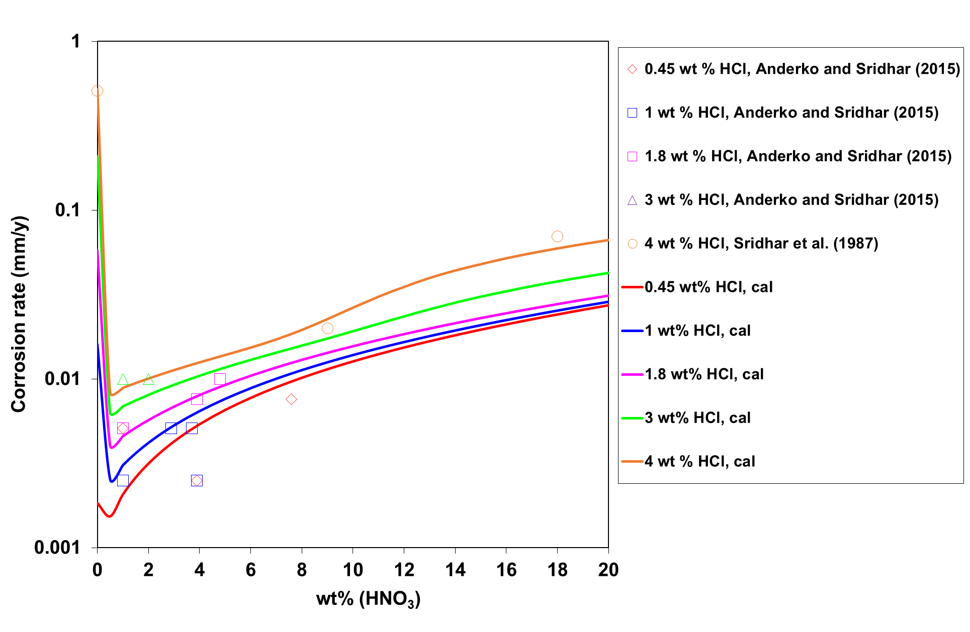 Figure 3: Calculated (lines) and experimental (symbols) effect of HNO3 concentration on corrosion rates of UNS N06022 in HCl + HNO3 mixtures at 353 K and fixed HCl concentrations.
A reverse effect, i.e., that of adding HCl to HNO3 solutions is shown in Figure 4 for UNS N10276. In this case, high HCl concentrations can destroy passivity and lead to very high corrosion rates. This phenomenon is due to the combined influence of a high corrosion potential resulting from HNO3 reduction, higher acidity due to the presence of HCl and shift in the passive current density that eventually establishes the mixed potential in the transpassive region.
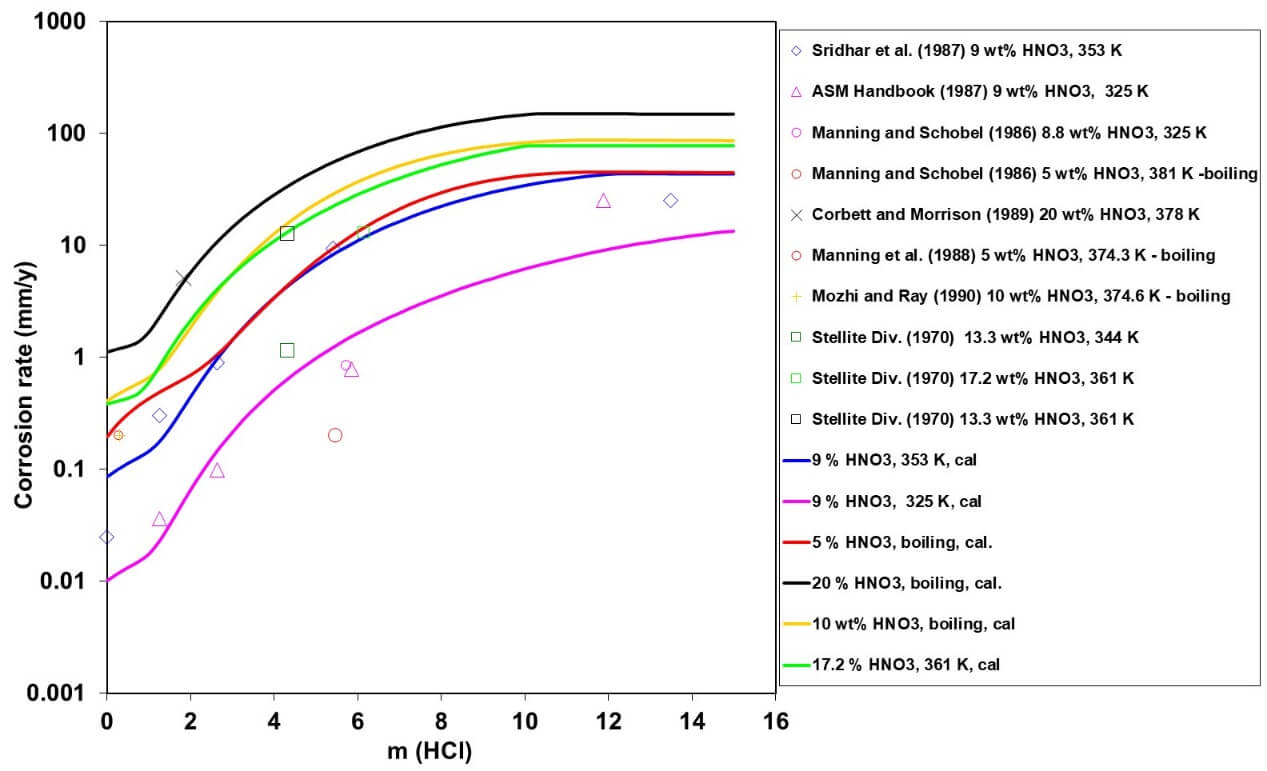 Figure 4: Calculated (lines) and experimental (symbols) effect of HCl concentration on corrosion rates of UNS N10276 in HCl + HNO3 z
aqueous mixtures at fixed HNO3 concentrations and temperatures ranging from 325 K to boiling.
Brines with or without oxidizing agents
Variation of the corrosion potential of UNS N06022 in aerated brine solutions is shown in Figure 5 as a function of pH. In the pH range from 2 to 13, the alloy is in the passive state and Ecorr is governed by the pH-dependence of the oxygen reduction. Such data, in combination with Ecorr data as a function of dissolved oxygen, are used to determine the properties of the oxygen reduction reaction, including reaction orders with respect to dissolved oxygen, exchange current density and the corresponding activation energy.
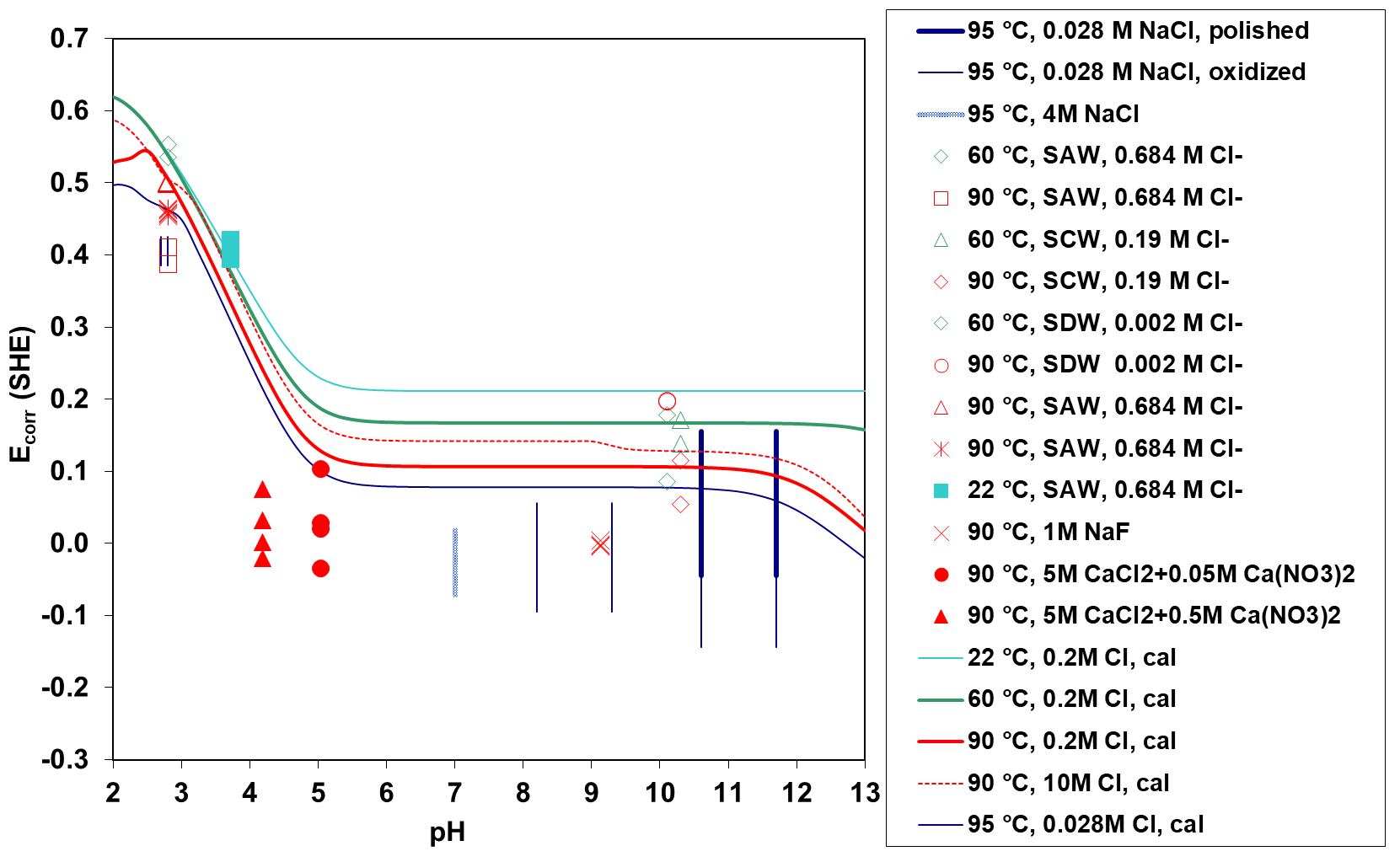 Figure 5: Calculated (curves) and experimental (symbols/vertical lines) corrosion potentials for UNS N06022 as a function of pH in aerated brine systems (SAW, simulated acidified water; SCW, simulated concentrated water; SDW, simulated dilute water). Vertical lines represent the ranges of the corresponding experimental data.
Depassivation pH is a practically important characteristic parameter that determines the range over which an alloy can be expected to be passive. To study the applicability of the model to predict the depassivation pH, Figure 6 shows the corrosion behavior of two types of UNS S41425 in a highly concentrated NaCl solution as a function of pH. The model can accurately represent the depassivation pH at 90 °C where a sudden drop in corrosion potential occurs and, consequently, high corrosion rates are expected. At higher temperatures, depassivation is expected to take place at higher pH values. This is predicted by the model at 150 °C (Figure 6). In addition, a comparison of the calculated Ecorr with Erp reveals the possibility of localized corrosion in narrow pH ranges from 2.2 to 2.4 and from 2.4 to 2.6 at 90°C and 150°C, respectively. The predicted slight susceptibility of UNS S41425 to localized corrosion is consistent with experimental observations.
The Erp values, which have been predicted based on a separate set of experimental data, show a very slight variation in the studied pH range. The small differences between the depassivation pH values reported by Cheldi and Scoppio (1999) are probably due to different Mo contents of two types of UNS S41425 used in their experiments.
 Figure 6: Prediction of depassivation pH and the possibility of localized corrosion for two types of UNS S41425 in NaCl aqueous solutions.
Concluding remarks
The OLI corrosion model computational framework has been parametrized and applied to study the corrosion behavior of various corrosion-resistant alloys in environments relevant to the chemical process industry. The model has been shown to reliably reproduce experimental corrosion rates in single or mixed acid solutions including both oxidizing and non-oxidizing acids. The model is also able to accurately calculate the corrosion potential in aerated brines over wide ranges of chloride concentrations. This includes the prediction of the depassivation pH, which can be used to estimate the passivity range in chloride solutions up to relatively high temperatures.
What tools are available for predicting corrosion?
The OLI corrosion model, which consists of a thermodynamic framework + a mechanistic model, is available in OLI Corrosion Analyzer V11 and OLI Studio V11.
Contact OLI at https:/www.olisystems.com/contact-us for more information or to schedule a meeting with an OLI expert.